Classifying Accents from Audio of Human Speech

This blog post details my second project completed while studying at Metis. The code for this project can be found here.

Project Overview

The guidelines for this project were as follows:

• Create a SQL database to store all tabular data. Make queries from this database to access data while performing analysis and modeling.
• Choose a project objective that requires use of supervised classification algorithms. Experiment with Random Forest, Logistic Regression, XGBoost, K-Nearest Neighbors, as well as ensembling any combination of models.
• Deploy the model in a Flask application or other interactive visualization.

It took me a bit longer than expected to decide on a project. I found myself stuck in a mental loop:

1. Search for interesting datasets.
2. Find something promising that would be a suitable binary or multi-classification problem.
3. Realize that the dataset had been downloaded by thousands of people, has been used in large Kaggle competitions, etc.
4. Self-doubt. (“Is my project original enough? Will it stand out?”)
5. Repeat.

Eventually, I was able to convince myself that as long as I pick something of interest to me and do a good job of applying what I had learned, it could be a successful project…but in all honesty it was the time limit that helped me to decide. This experience taught me the balance between thoughtfully planning a project, but still efficiently delivering a useful MVP on a deadline. It’s more important to finish a simple yet useful project than come up empty handed with an overly complex or over-perfected project.

My project objective was to classify spoken audio of speakers from six countries as American or not-American. (This was the result of narrowing the scope of my initial project objective, as explained in Obstacles below.)

The Dataset

I used the Speaker Accent Recognition Dataset from the UCI Machine Learning Repository. This dataset includes data extracted from over 300 audio recordings of speakers from six different countries. Half of the data contains speakers from the United States, and the other half is divided among Spain, France, Germany, Italy, and the United Kingdom. (The original paper is referenced in References.)

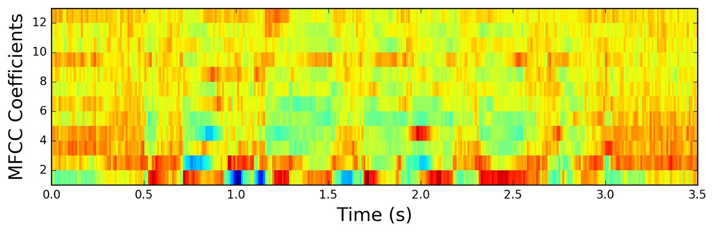
Each audio recording in this dataset was pre-processed and transformed into 12 Mel-frequency Cepstrum Coefficients (MFCC).

The data was easy to acquire (a simple .csv download). However, in order to add a learning element to the project, I created a SQL database on an AWS EC2 instance to store the data and access it remotely.

Obstacles

Modifying Initial Scope

Similarly to my last project, I had to iteratively modify the scope. Initially I intended to create a multinomial classifier for all of the accents present in the dataset, but the data was too limited. Not only was the total size of the dataset particularly small, but this was further compounded by the class imbalance between American accents and all other accents. Unsurprisingly, I pivoted towards creating a binary classifier to distinguish between American and all other accents.

Inability to Reproduce Features

I had hoped to increase the sample size of non-American accents for each by transforming audio from the Speech Accent Archive into MFCC features. However, I was unable to reproduce the existing data with a couple of different Python packages (librosa and python-speech-features). Therefore, I wouldn’t have been able to trust the results of applying these packages to new audio recordings. This further contributed to the need to narrow the scope of the project to a binary classifier.

Interpretability of Features

Due to the esoteric nature of the field of psychoacoustics, MFCC features are not interpretable to most people (including myself). If I told you that “an accent being American is dependent on the 10th MFCC”, that would be effectively meaningless. This was unfortunate for two reasons:

1. I couldn’t intelligently and creatively do feature engineering to improve my model. Using a more brute force feature engineering approach was somewhat helpful, but having some domain specific knowledge is advantageous.

2. The classifier itself wasn’t interpretable. In other words, I couldn’t draw any useful conclusions on the relationship between particular MFCC and particular accents.

Modeling & Results

Before beginning any modeling, I trained the original dataset on K-Nearest Neighbors, Random Forest, and Logistic Regression and recorded their training and validation ROC AUC scores to serve as a set of baseline models.

Exploratory Data Analysis & Feature Engineering

The data was of high quality and minimal cleaning was necessary so I moved quickly into exploratory data analysis. Upon plotting the distributions of each feature (separated by class), I noticed that some features had bimodal distributions for only one class.

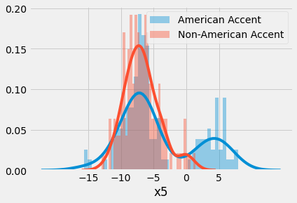
For features like x5 [unitless], the distribution for instances where the labeled called was “American” has a distinct second mode.

I tried adding an additional boolean feature that indicated if a particular feature was in its respective bimodal range to try and put more weight on that behavior in the distributions and sort of “enforce” the separability in the data. Unfortunately this didn’t improve the ROC AUC scores or overfitting of the baseline models.

I then automatically generated all interaction terms between the original features and plotted their feature importances.

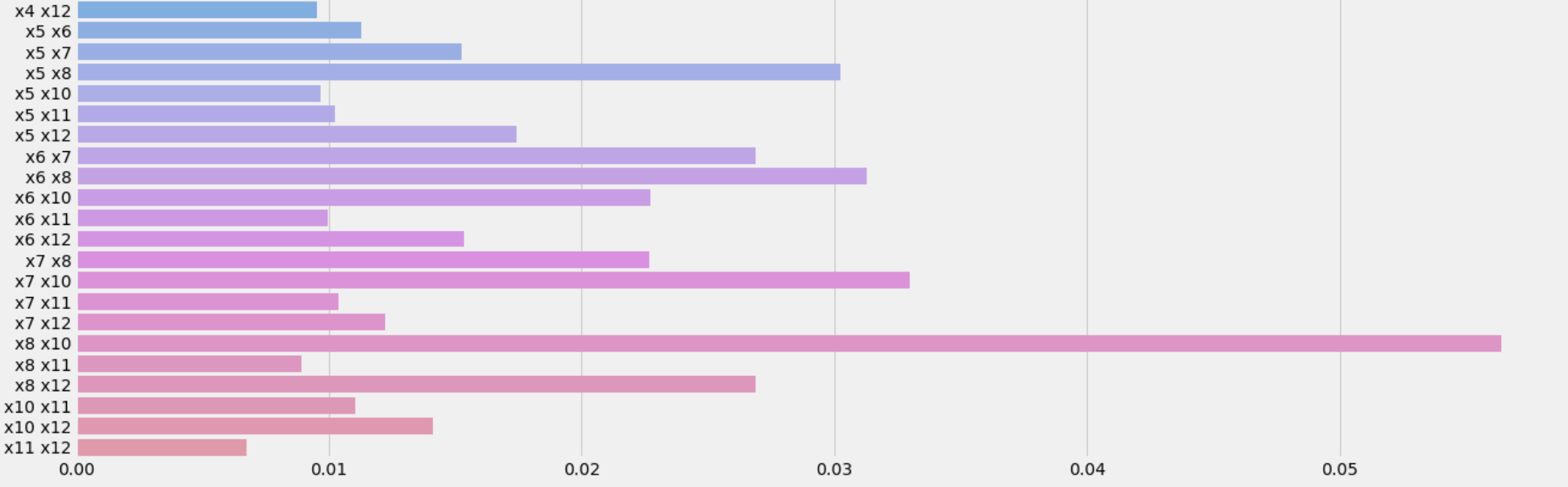
A subset of the interaction features’ importances.

I used the information gained from the feature importance graph to add various interaction features, but eventually realized that simply removing x9 (one of the original MFCC features) yielded the best improvement in ROC AUC as compared to the baseline model.

Model Selection & Tuning

The next step was to tune the hyperparameters on each baseline model, using the final set of selected features, to achieve the best ROC AUC scores and least overfitting for each. This was all done using models in scikit-learn. For the Logistic Regression model, tuning involved:

• Running the model with both L2 (Ridge) and L1 (Lasso) regularization.
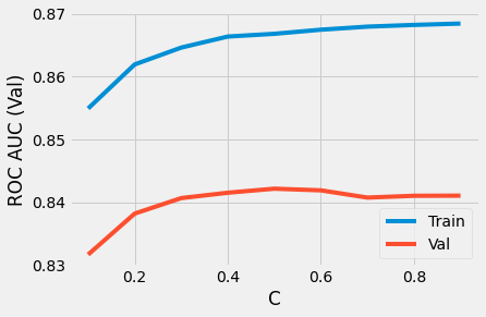
• Optimizing the inverse regularization strength to strike a balance between maximizing the ROC AUC validation score and reducing overfitting (minimizing the difference between the training and validation ROC AUC scores.)

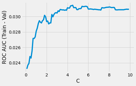
The difference between training and validation ROC AUC scores with respect to inverse regularization strength.

The training and validation scores plotted separately.

This analysis resulted in a Logistic Regression with L1 regularization and C = 0.1 which successfully reduced overfitting to a negligible amount while retaining a good ROC AUC score of 0.85.

The K-Nearest Neighbors (KNN) model was optimized using similar metrics, but using instead the “number of neighbors” hyperparameter. The optimal KNN used 6 neighbors and resulted in an ROC AUC score of 0.92, with reduced overfitting.

Finally, for the Random Forest I tweaked the number of estimators, max depth, and maximum number of observations per leaf. The best Forest yielded an ROC AUC score of 0.83.

Among these three models, the KNN performed the best. However, I wanted to try ensembling different combinations of these three models to see if I could outperform the individual KNN. It turned out that the best model was an ensemble of the KNN and Logistic Regression, determined by examining a more detailed set of scores including accuracy, precision, and recall of the classifier.

Bonus: I also played around with XGBoost, but had limited time to optimize the hyperparameters and was satisfied enough with the performance of my existing ensemble model.

Threshold Tuning

Classification models in scikit-learn use a threshold of 0.5 by default to classify predicted probabilities as the positive class (for probabilities above the threshold) or the negative class (for probabilities below). However, by changing the threshold, it is possible to get better accuracy out of your model.

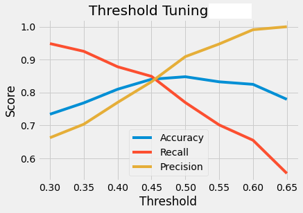Performance of model at different thresholds.

A threshold of 0.46 yielded negligible change in accuracy while providing a slightly better balance between precision and recall.

Final Scoring

Scoring the final model on the test set yielded an overall accuracy of 0.89. I chose accuracy as the main scoring metric because in the case of classifying accents, there’s no reason to optimize precision or recall (whereas you might care more about these metrics in higher risk domains such as medicine.)

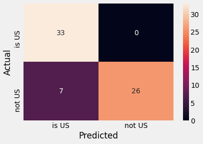Test set confusion matrix of final model.

Flask App

I deployed the model in a Flask application on Google App Engine Heroku (migrated because it was cheaper). The app allows you to select audio examples of each accent, listen to the sample, view it’s MFCC coefficients, and play around with them to yield different predicted classes (accents).

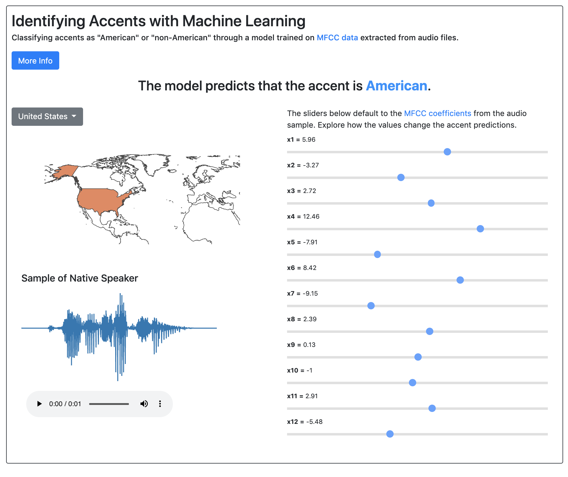Screenshot of the Flask application.

Summary

I learned a couple of important things from completing this project:

1. It’s important to understand the limitations of your dataset before going too far down an impossible path. In my case, it was wise to quickly switch to a binary classification after realizing how small and imbalanced my dataset was.

2. Methodically working through model selection and tuning in an organized fashion can lead you to a model you are happy with. It can help you avoid the infinite loop of model tweaking.

References

Fokoue, E. (2020). UCI Machine Learning Repository - Speaker Accent Recognition Data Set. Irvine, CA: University of California, School of Information and Computer Science.