Predicting Popularity of Hip-Hop Music on Spotify

Disclaimer: Much of this post assumes that the reader has some basic data science knowledge, as opposed to my inaugural post which was a self-reflective, career oriented post.

I just completed the first major independent project during my time as a student at Metis. We were given two weeks to complete a project that satisfied the following constraints:

• Train a model that predicts a continuous, numeric value using a mix of numerical and categorical data.
• The model must be fit using only linear regression, polynomial regression, or any regularization-enhanced variant of linear regression (Lasso, Ridge, ElasticNet).
• At least a portion of the training data must be acquired via web-scraping.
• Use a relatively small training set (on the order of 100’s or 1000’s of records).

Generally, I enjoyed working through the full data science workflow for the first time and being able to go deep into a data set. This blog post details my process, from the initial search for data to deploying the model.

Motivation

My opinion going into my first project was that aside from all technical metrics, there are two determinants of a compelling portfolio project:

1. The project should use a topic/data set that excites you. That excitement and passion will come through in your work.
2. The project should not just produce “interesting” or “cool” results. The results should be actionable and carry value. Your future hiring manager might like to see something that is fun, but they also most likely want to see that you can make valuable predictions and/or interpretations with data.

As a music producer and someone exploring music technology as a potential career path, I felt compelled to search for music-related data. I find the field of music recommendation and personalization to be exciting. Reading the Spotify Engineering blog gave me the prior knowledge that they are on the cutting edge of music technology, and that they publish interesting, high-quality data sets on their API. One particular Spotify data set that stood out to me contains “track audio features”. These data are generated by a proprietary algorithm for every track on the Spotify platform, and contain such features as “danceability”, “energy”, and “loudness”. Most of these features are numerically encoded on a scale of 0 to 1.

As far as yielding valuable conclusions, it seemed that the best way to apply this data was to predict the success of a song based on its various qualities and what factors carry the most weight. Choosing a target to predict that accomplished this goal took some time, but was a good lesson in selection of project scope.

Narrowing the Scope

Initial Scope

The first thing that came to mind to predict was Pitchfork album ratings. Pitchfork is arguably the most well-established music blog on the internet. The website’s most prominent feature is its album reviews, each of which contain a written review and a rating, scored on a scale of 0 to 10. While these reviews have received heavy criticism and scrutiny, their stamp of approval has been credited with jump starting the successful music careers of artists like Arcade Fire and Bon Iver. Surely, a good review on Pitchfork is a strong indicator of (and sometimes reason for) a successful album.

However, initial exploratory data analysis showed that Pitchfork album rating might not be a promising target variable,
for two main reasons:

When plotting all of my feature data against Pitchfork album rating, there was no obvious relationship. Could I have chosen new features? Maybe, but I really was enjoying exploring the Spotify audio feature data, and believed that there was some value in it.

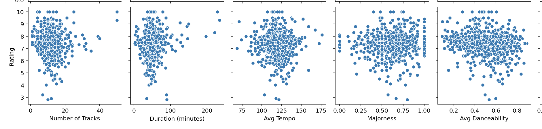
Pitchfork Album rating plotted versus a few track audio features/metadata, showing very little feature-by-feature correlation with the target.

Running a baseline Linear Regression model on the data yielded a validation R-squared score of 0.091, which felt too low to do extensive feature engineering and training on given the time constraint.

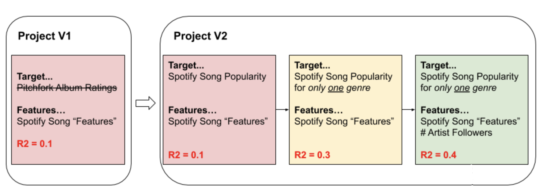
The process of choosing an appropriate project scope.

Why was this model performing so poorly? If you remember, the Spotify audio features are available for individual tracks, but the Pitchfork ratings are for albums. I had to do some data processing to aggregate the track-level audio features as album-level features, which mostly amounted to taking averages across the album. My suspicion is that since an album can contain songs with varied “vibes”, averaging features like “energy” and “danceability” neutralized the significance of these metrics. Beyond that, it seems that album reviews and ratings are highly subject to the tastes of the person writing a particular review, or perhaps what side of the bed they wake up on that morning. Something so subjective is unlikely to show a clear pattern in the data.

If I was being asked by an employer or client to specifically predict Pitchfork Album Ratings, I would have persisted. While I’m looking forward to having a job, being a student gave me the flexibility to pivot my project slightly.

Setting a New Target

My next objective was to find a track-level feature that in some way represented commercial success. Spotify, being the good data stewards that they are, provides a “popularity score” for each track on their platform via the API. Spotify doesn’t provide documentation on how they calculate popularity, a score given on a 0-100 scale, but they do state that it is highly dependent on the number of streams a track has, and how recent those streams are - in other words, how “hot” or “viral” a track has been. Once again, by creating a pair plot of the new target (popularity), I saw no obvious correlations and knew that I hadn’t quite hit the mark on my project scope. Running another baseline linear regression model doubled my previous R-squared score to around 0.2, but this still didn’t seem like a good starting point for feature engineering and tuning, given my relative lack of exposure to those skills at the time.

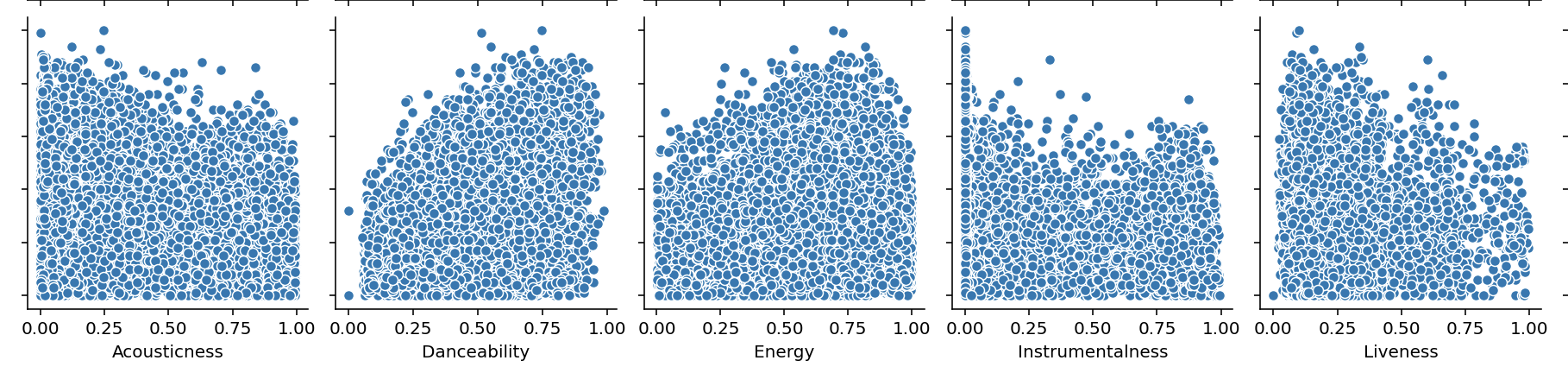
Popularity plotted versus a few track audio features/metadata, showing very little feature-by-feature correlation with the target.

Choosing the Final Scope

It was then that I learned the value of stepping away from the Jupyter Notebook for a few minutes to think about the problem at hand from a practical, common-sense perspective. “Different genres of music are popular for different reasons, right?”, I thought to myself. For instance, a fan of Folk/Country probably won’t like a “danceable”, “high energy song”, but a fan of electronic music might. Fortunately, I already had a column for genre in my data set, so I separated the data into each genre and plotted a correlation matrix for each. Hip Hop music showed the most highly correlated features, so I made the decision to finalize my scope, and title my project, “Predicting Popularity of Hip Hop Music on Spotify”. I did some data cleaning on the filtered hip hop data, and persisted my data set in preparation for the next phase of the project.

Feature Engineering, Modeling, & Technicals

The first way I improved the baseline model was through a new features and feature engineering. Both of these tasks can take you into deep rabbit holes - given the time limit, I decided to set a reasonable goal of adding at least one brand new column of data, and one new feature created by transforming an existing feature or combining features.

Feature Addition: Artist Followers

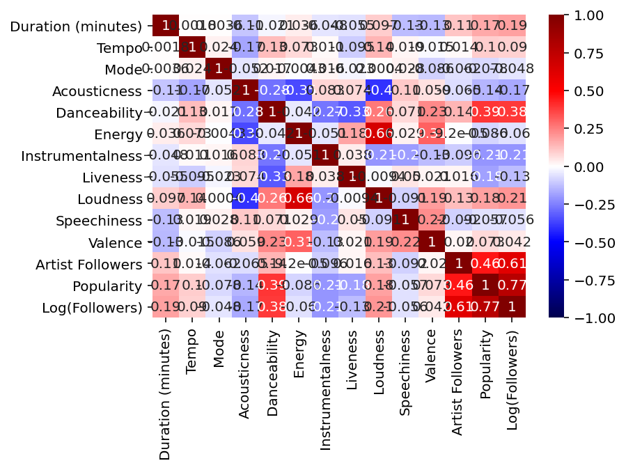
While Spotify’s definition of song “popularity” implies that even up and coming artists can have very popular songs, artist follower count (available via Spotify’s API) still sounded like a strong contender for predicting song popularity. After querying Spotify’s API for each artist of each song and adding the number of followers as a column to the data, I plotted a correlation matrix:

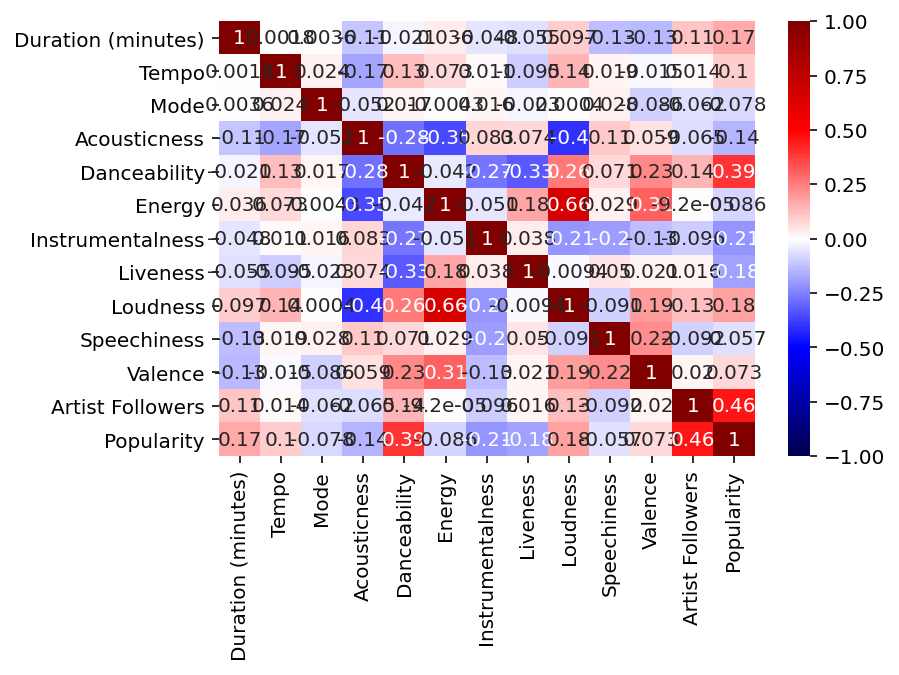
Correlation matrix of data after adding number of artist followers as a feature.

Sure enough, artist followers was the most highly correlated feature.

Feature Engineering: Log Transforming Artist Followers

The feature I added turned out to be the feature I engineered. Upon inspecting the plot of popularity versus artist followers, I noticed that the relationship could be fit to a logarithmic equation (log(x)).

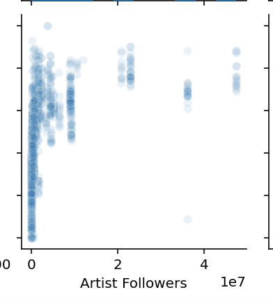Song Popularity vs. Artist Followers, a sparse, but logarithmic relationship.

Log transforming the feature (taking the log of artist followers) yielded a relatively strong linear relationship.

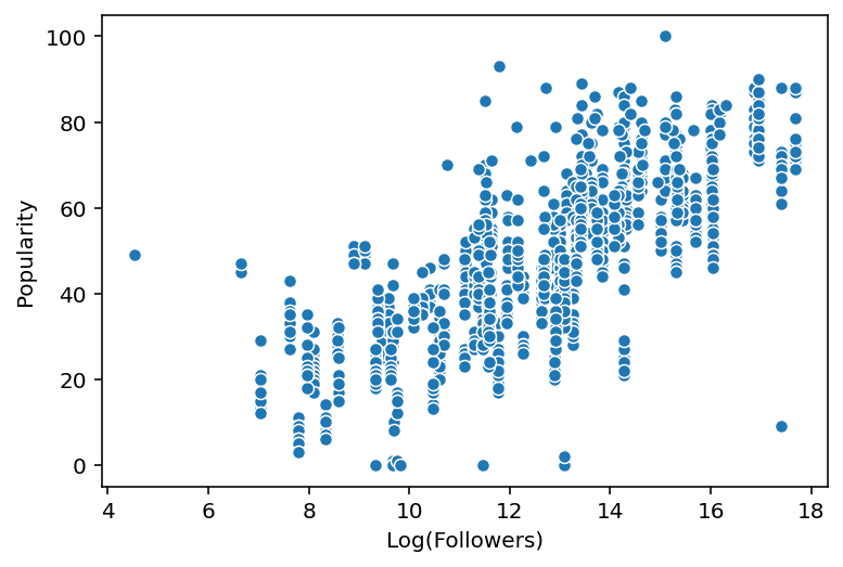Song Popularity vs. the Log of Artist Followers, showing a linear relationship.

Finally, plotting the correlation matrix with the addition of Log(Artist Followers) shows a more highly correlated feature to use in a model that predicts song popularity.

Modeling & Evaluation of Metrics

I began developing the final model by splitting the full data set into a training/validation (train-val) set (75% of data) and test set (25% of data). Running cross validation on a linear regression model using the train-val set yielded a training R-squared score of 0.61, a validation R-squared score of 0.58, and a root mean square error (RMSE) of 12.29.

In an attempt to reduce model overfitting, I ran both a Lasso and Ridge regression with varying regularization parameters (alpha). Both yielded similar best results of a training R-squared score equal to 0.62, validation R-squared score of 0.61, and similar RMSE to the baseline linear regression. Both models succeeded in reducing complexity and raising the validation R-squared score, without affecting RMSE.

From there, I experimented to see if I could raise the R-squared score and lower RMSE. I tried a combination of polynomial regression and Lasso regression to eliminate unneeded polynomial features, which yielded very similar results. Since the coefficients of polynomial regression are harder to interpret than linear features, and there was no improvement in model performance, I threw the model out.

Another experiment I tried was pre-removing the features from the dataset that the initial Lasso removed (by reducing their coefficients to zero). I then ran additional Lasso and Ridge regressions on that dimension-reduced feature set to see if that had any effect on the model performance. This also yielded similar results, so I decided to go with the model that I felt would be the easiest to interpret. The Lasso model, run on the reduced feature set, left me with a model with reduced complexity from the original baseline regression, and a slightly reduced feature set. It had a few slight advantages: a validation R-squared score on the higher end of all of my models (0.619), the smallest difference between training R-squared score and validation R-squared score (0.05) indicating very little overfitting, and an RMSE on the lower end of all of my models (12.1).

Scoring the model on the test set yielded a final R-squared score of 0.579 and RMSE of 13.8, indicating that on average the predictions of song popularity are off by 13.8. If an artist is trying to determine if their song will be popular a score of, for instance, 70 out of 100 might be, in some cases, anywhere from 57 to 83. Based on my understanding of the distributions of popularity on Spotify, even a score on that lower end indicates a successful song. This model could be improved quite a bit, but still provides potential value for hip hop artist trying to predict the impact of their music.

As an additional quality check on the model, I evaluated a few of the essential linear regression assumptions:

1. The residuals have a fairly constant variance for all predictions.
2. The predictions are approximately normally distributed.

Final Steps

Deploying the Model

After scoring the final model, I challenged myself to create a simple web application (using Streamlit) that allows anyone to play around with the model parameters and make predictions.

As a final bonus, I learned how to make a Dockerfile for the application and deploy it to Google Cloud App Engine. Update (2020-09-17): I’ve since migrated the app to Heroku because it is much cheaper.

Lessons Learned

Aside from the theory and technical skilled learned, I took away a couple of general lessons from this project:

• Refining scope can lead to a much more successful project, model, or product.
• When feature engineering and model tuning gets tedious, take a step back and think about the problem at hand from a more global, common sense perspective.

The code for this project can be accessed here.

The Streamlit app I created for this project can be accessed here.