Object Detection for Autonomous Snow Grooming Applications

This post is a technical overview of my Metis capstone project, completed over a 3-week span. I developed a proof of concept for autonomous snow grooming vehicles at ski resorts. I accomplished this by training a Faster R-CNN object detection model in PyTorch to detect/classify obstacles in dash cam footage from vehicles moving through a ski resort.

The code for this project can be found here.
Note: There is a button within the .ipynb file on GitHub to open it in an interactive Google Colab environment.

Motivation & Objective

This was a completely open-ended project - we were simply told to choose a “passion project” in any subdomain of machine learning. I was overwhelmed with the task of choosing from an infinite project space, but quickly asked myself a simple question to narrow down my options: What machine learning realm did I most want to explore that hadn’t yet been covered in the curriculum? The answer was Computer Vision.

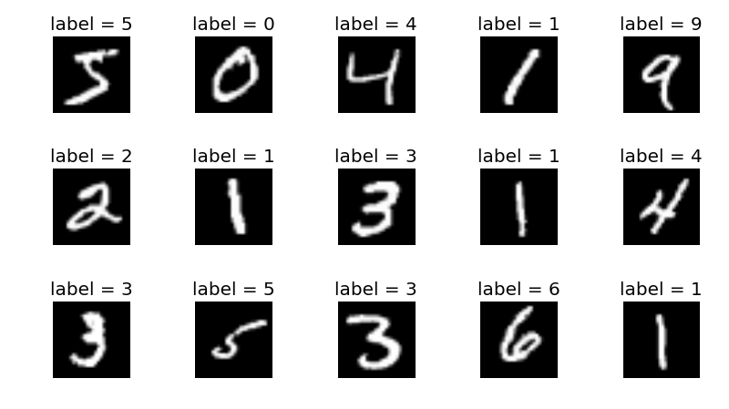
MNIST handwritten digits dataset, commonly used for introducing image recognition concepts. (Image: Towards Data Science)

Yet, even computer vision is a vast field of study. I thought back to the Metis curriculum, when we reviewed a relatively simple application of convolutional neural networks (CNN) to perform image recognition (via the classic MNIST handwritten digits dataset). However, I wanted to build on top of that knowledge and challenge myself with something more complex. The logical next step seemed to be object detection.

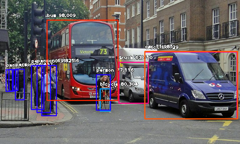
An example of object detection in autonomous vehicle applications. (Image: Towards Data Science)

I knew that object detection was one component of autonomous vehicle technology, but I felt hesitant. There are a lot of open source autonomous vehicle datasets out there, but I didn’t feel like I could extract any more value than the thousands (?) of people with PhD’s in computer vision that had already done so.

This was the point at which I considered some of my extracurricular passions. I happen to really enjoy skiing. If you’ve ever been to a ski resort, you might have seen a large vehicle that looks like some combination of a snow plow and a military tank. These are “snow cats” - continuous track vehicles designed to move on rugged, snowy terrain. Snow cats are sometimes used for transport, but are mostly used as “snow groomers” at ski resorts. Snow grooming vehicles smooth and move around snow to make the mountain safer and more enjoyable for skiers and snowboarders. They operate nightly, and also sometimes during the day to keep the mountain open when there is heavy snowfall.

A snow groomer. (Image: Pistenbully)

This felt like it could be a fun, novel application of autonomous vehicle technology. Snow grooming is expensive and potentially hazardous - both things that can possibly be reduced through automation. Furthermore, it is a well-defined problem in the sense that a snow grooming vehicle only has to be able to detect a narrow subset of obstacles as compared to a car driving on a busy city street. Due to the fact that autonomous vehicle software requires many different components (instance segmentation, trajectory planning, etc.), I defined my project as a proof of concept for autonomous snow grooming vehicles using only object detection.

The deliverables of this project were two-fold:

1. A neural network trained to detect objects in images that a snow grooming vehicle might see in its field of view.
2. A demo created by applying the model to snow groomer dash cam footage to draw boundary boxes around detected objects.

Methodology

Object Detection

An object detection model is designed to return two sets of outputs for a given image:

1. The detected instances of semantic objects of a variety of classes in the image (ex. “tree”, “person”, “car”).
2. A set of Cartesian coordinates describing the boundary boxes of each detected object in units pixels.

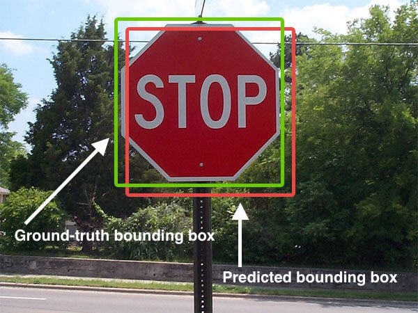
Boundary box for a stop sign in an image. (Image: PyImageSearch)

Therefore, it follows that the training data for such a model must contain “ground truth” boundary boxes with annotated class labels on each image.

Data

It turns out that it is extremely labor intensive to manually draw boundary boxes on thousands of images. In fact, it is common for companies tackling computer vision problems to out source the annotation/labeling task to “mechanical turks” - a.k.a. humans paid per labeling task they successfully complete. New start-ups have sprouted up to specifically provide labeling services.

Luckily, the open-source community once again provides, in the form of pre-annotated datasets for object detection. I decided to use Google’s Open Images Dataset via the openimages Python library. This dataset contains images as well as corresponding .xml files containing the object classes and boundary boxes for each image. This required me to write an xml parser to extract the boundary box information, but was generally an easy dataset to interact with.

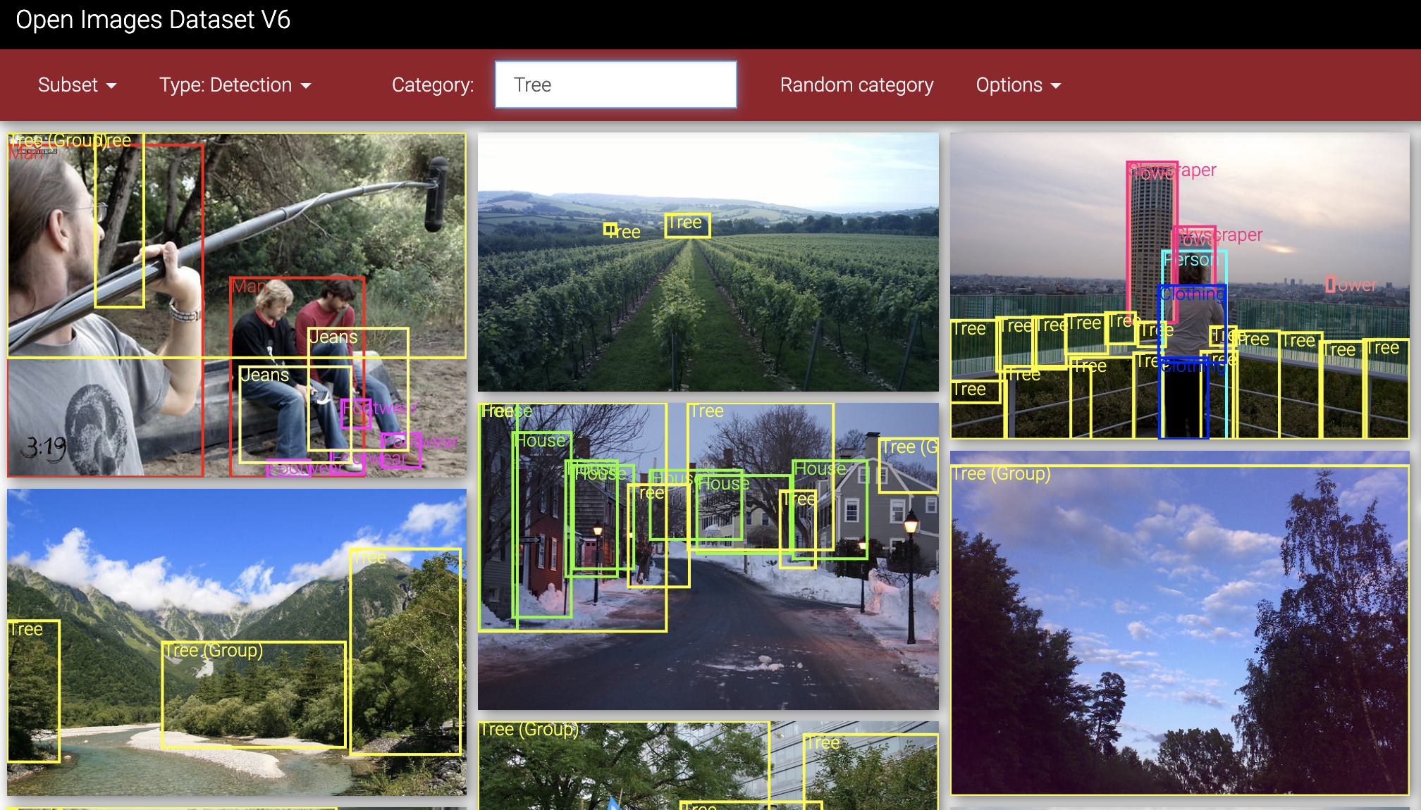
Annotated images from Google Open Images Dataset.

While I initially wanted to detect up to ten different classes, I ran into performance issues that I couldn’t remedy in the short term. The trade-off was: create a model that predicts many object classes with low confidence, or one that predicts fewer object classes with higher confidence. I chose the latter option which resulted in three object classes for the model to detect:

• Person
• Tree
• Ski Lift Pole (Note: The Google Open Images dataset only had images labeled “street light”, which look quite similar to the pole structure for a ski lift, so I assumed it would be a sufficient proxy. I turned out to be right: when presented with only images/video from a ski mountain, the model recognized poles as “street lights”. I simply renamed the class label in the .xml files from the dataset to “pole”.)

These three classes seemed like the most essential objects for a snow grooming vehicle to be able to detect as it moves up and down the mountain. I downloaded approximately 5000 images per class, some containing multiple object instances (for instance, 3 annotated trees in a single image).

Transfer Learning

The primary machine learning technique used for this project was transfer learning. In general, transfer learning involves taking a model already trained on a large dataset for some task and repurposing it for another task. More specifically, the process is as follows:

1. Take a pre-trained neural network architecture designed to perform a particular task.
2. “Freeze” most of the layers in the neural net so that their weights can’t be updated when training on a new dataset.
3. Replace the final (few) classification layer(s) so that it is both trainable and able to predict the number of classes specific to the new task.
4. Train the model on a custom dataset suited to the new task.

Transfer Learning (Image: Pennylane)

It may be obvious to some, but what are some reasons you’d want to use transfer learning?

• In the context of image classification/object detection, fine-tuning a neural net pre-trained on a vast image set allows your new model to take advantage of some general network “fundamentals”, such as layers that pick up on edges, shapes, and components of a particular object in an image. The final model adds a layer that picks up more complex combinations of fundamental features that separate the various images/objects.
• Since only a fraction of the weights of the neural network have to be updated with every training epoch, the model can be trained much more quickly.

Choosing the Right Tools

Determining which computing platform and neural network library to use took up the majority of my time while working on this project.

Computing Platform

Due to the fact that training neural networks on large datasets can be extremely CPU and RAM intensive, it is common to use a GPU on a cloud compute platform rather than a laptop. Unfortunately, I initially jumped to an overly complex option. I provisioned a server on Google Cloud (GCP), but quickly realized that this was too “heavyweight” and costly for my project, and shut down the server.

I ended up choosing to work with the popular Google Colaboratory. This platform, allows you to freely run software on GPUs using a coding interface based on Jupyter Notebook, and host and access data on a Google Drive folder.

Neural Network Toolkit

As most people in the data science community are aware, the two most popular neural network libraries written in Python are Google’s TensorFlow and Facebook’s PyTorch. I initially began to work on this project using Keras (a simplified API within the TensorFlow library), simply because that’s the library we had used in demos while learning about neural networks at Metis.

I wasn’t able to quickly achieve a workable prototype of my model using TensorFlow. I still am not 100% sure why this happened, since everything I knew about TensorFlow indicated its vast capabilities. It could have been that TensorFlow actually does have a steep learning curve, or that the tutorials available in their documentation are better suited for other tasks, or perhaps my lack of understanding in general. Due to the extremely limited time allotted for this project, I gracefully took the hit to my ego, and began to search around blogs and other documentation for a suitable solution.

I eventually stumbled upon the Torchvision Object Detection Finetuning Tutorial, which turned out to be the perfect starting point, and led me to choose PyTorch as the primary toolkit for this project. (That being said, there was still a decent amount of work necessary to adapt the tutorial such as ingesting a different data format, creating a custom torch.utils.data.Dataset class, removing the “Mask R-CNN” model for instance segmentation, adding custom image transformations for training, and much more.)

Auxiliary Computer Vision Tasks

Demo-ing this model on video footage required the auxiliary task of drawing predicted boundary boxes and labels on each frame. The choice to perform this task was a bit more obvious - OpenCV. OpenCV is one of the most popular libraries in the computer vision community. In addition to containing libraries for image augmentation, it also has its own machine learning modeling libraries. I used the Python implementation of OpenCV, opencv-python to carry out the boundary box drawing task.

Training the Model

I would have liked to spend a lot more time trying out different optimizers and hyperparameters for the model, but given the time constraint I settled on a model with the following features:

• The base model was a Faster R-CNN with ResNet architecture, pretrained on the COCO Image Dataset (>200,000 images containing ~1 million object instances from 80 different object classes).
• The neural network was frozen up until the last 3 backbone layers allowing their weights to be fine-tuned on the custom “ski resort” dataset.
• 80% of the data was allocated to training/validation, and 20% was allocated to testing. Within the training/validation set, it was split 80% for training, 20% for validation.
• The model trained for up to 10 epochs, with a stopping condition in place if the validation score started to rise after continuously falling for some number of epochs.
• I used an initial learning rate of 0.0001 with a learning rate scheduler set to decrease the learning rate by a factor of ten every 3 epochs.
• Stochastic Gradient Descent (SGD) with a momentum of 0.9 was used as the optimization algorithm. I tried using ADAM, but that yielded lower performance.
• The loss function being minimized by SGD is the Smooth L1 Loss or “Huber” loss.

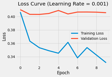
Training and Validation scores for each of the model’s training epochs.

In order to assess overfitting I plotted training loss and validation loss for every epoch. By the time the project was due, the model was still too complex. If I had more time, I would have:

• Experimented with introducing dropout layers.
• Experimented with removing some layers in the network to reduce complexity.
• Trained using a larger dataset.
• Leveraged more compute power to do k-fold cross validation to determine the optimal set of hyperparameters.
• Specifically messed around with weight decay (L2 regularization) to try and reduce model complexity.

Evaluating the Model

Quantitative Evaluation

As described earlier, object detection training data is composed of images, boundary boxes, and labels. A given image may contain multiple detectable objects, and its corresponding annotation will indicate the class of those objects (ex. “tree”) as well as pixel coordinates indicating the bounding box of each object. The boundary box label and coordinates provided in the training/testing data is ground truth. Once an object detection model is trained, it will output a set of predicted boundary boxes for any image it sees.

In order to score the performance of the model, we need some kind of metric to compare predicted and ground truth boundary boxes/labels for every image in the test set. Intersection of Union (IOU) partially serves this need by calculating the area of overlap divided by the total area that both boundary boxes take up in space. If the predicted box were to exactly line up with the ground truth box, then IOU = 1.

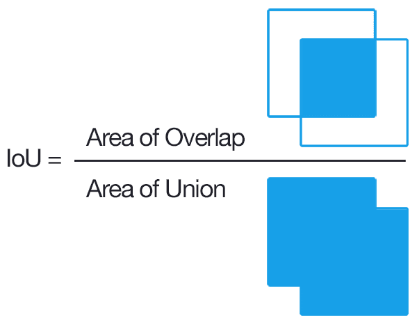
Intersection of Union (IoU) Calculation (Image: PyImageSearch)

However, this isn’t the final metric used to score the performance of the classification model. The evaluator function calculates mean precision and recall across all test images at various IOU’s and ranges of IOU’s. So, for instance, it will output the mean average precision (mAP) for all boundary box predictions that achieved between 0.5:0.95 IOU with their respective ground truth boundary box. This way of calculating accuracy-type metrics allows for some flexibility in how the user chooses to evaluate the results. For instance, if all I care about is generally detecting that something exists in an image, I might accept a precision score at an IOU of 0.5. However, if that objects exact location in space is important, I might look more at metrics evaluated at an IOU closer to 0.95.

My model achieved a mAP of 0.178 and a mAR of 0.319 for an IOU threshold range of 0.5:0.95. For reference, the original object detection model that I applied transfer learning to achieve a mAP of 0.37 on the COCO image dataset.

Qualitative Evaluation: The Demo

In order to simulate the performance of the model on an actual snow grooming vehicle, I found some dash cam footage from snow cats and go pro footage from skiers moving through a mountain. I used OpenCV to separate the videos into frames, applied the model to each frame and drew predicted boundary boxes, and stitched the frames back together into a video. This was the result:

Qualitatively, the model is able to detect trees, people, and poles. This demo revealed one major point of future improvement in the model: it is unable to distinguish “groupings” of objects relative to individual instances. It would be important for an autonomous snow grooming vehicle to be able to make this distinction. Upon further investigation, it turned out that the dataset I used actually indicated whether a ground truth bounding box applied to a group or single instance. This is something that could definitely be incorporated to improve the model in the future.

API

With just a bit of time to spare before the final presentation, I decided to prototype an API that contains an endpoint for making object detection predictions on any image. I didn’t spend time deploying it to a server, but it can be run on localhost. (See instructions on how to use it here.)

Below is the presentation I gave on this work for my capstone project at Metis. It is a high-level overview of what was discussed in this blog post.

Recommender Systems are a Joke - Unsupervised Learning with Stand-Up Comedy

Disclaimer: This post as well as the code accompanying it contains some direct and indirect references to potentially offensive language. This is an analysis of stand-up comedy, which tends to contain curse words, racial slurs, etc. However, all references are made with objective, academic intent. If you have any concerns with my treatment of certain language, I’d be happy to have a conversation. You can get in touch with me via LinkedIn.

This post documents my first foray into unsupervised learning, natural language processing, and recommender systems. I completed this project over a 2-week span during my time as a student at Metis.

The code for this project can be found here. The Flask app I made for this project can be found here.

Intro

Comedy! (Image: Scraps from the Loft)

A little over halfway through the Metis data science bootcamp, the curriculum shifted from supervised to unsupervised learning. At that point, my brain was
firmly in “predict y given X” mode, and it quite honestly took a few days to wrap my head around what it means to use machine learning on unlabeled data, and why that would even be useful. It clicked when I applied a rudimentary model of the human brain to both of these approaches: often our brains make inferences based on our previous experiences and knowledge (supervised learning). However, sometimes we are forced to find previously unseen patterns in the world around us (unsupervised learning) before we can make decisions.

Concurrently, we were introduced to Natural Language Processing (NLP). In addition to learning a lot specifically about NLP, one big takeaway was a clearer understanding of what is meant by “Artificial Intelligence” in the context of machine learning - any instance of a computer being able to imitate (or even replicate) a human perception or ability. After this realization, I went from being somewhat weary of apply machine learning to text/speech, to extremely motivated to work on an NLP problem.

As you might expect, the main requirements of this project were:

1. Use unsupervised learning.
2. Use text as the primary data source.

I almost instantly came up with an idea. Stand-up comedy specials are usually in a 1-hour monologue format, and are rich and diverse in topics, opinions, colloquialisms, and regional english dialects. For that reason, and also the fact that I’m a huge fan of the comedy world, I knew that this would be a stimulating project.

Data Wrangling

Luckily, I was able to quickly find a website (Scraps from the Loft) with several hundred comedy transcripts. I used the Python requests) library in a script to acquire all of the raw HTML for each transcript, and Beautiful Soup to parse the main text and various metadata (comedian, title of comedy special, year).

After inserting the data into pandas dataframes (one for the metadata and one for the text corpus), I stored it in a remote Mongo database on an Amazon AWS EC2 instance. Admittedly, this wasn’t really necessary as my corpus was small enough to store locally , but I wanted to get more comfortable with both creating MongoDB collections and querying data for analysis and modeling using pymongo.

Data Cleaning & The NLP Pipeline

As we had been warned, cleaning and preparing the text corpus proved to be the most critical, time consuming part of this project. Topic modeling (and clustering) of text data relies on sufficient elimination of extraneous words, but also careful inclusion of words that might be indicators of a topic.

First, I performed some “macro” cleaning, removing entire documents (individual transcripts) that would throw off the modeling and/or not be relevant in a recommender app. That involved removing:

• Comedy specials in different languages (there were a handful in Italian and Spanish).
• Comedy specials that are not widely available (or available at all) on streaming platforms.
• Short-form comedy such as monologues on Saturday Night Live, or other late night TV shows.

I then created an “NLP pipeline”, that can take any document from the corpus and perform the following transformations:

• Clean the text by removing punctuation, non-essential parts like the person introducing the comedian, removing numbers, removing line breaks, crazy noises and expressions like “aaaaah”, and common English stop words.
• “Lemmatized” words to reduce all forms of words to their base or “lemma”. (For example, “studies” and “studying” become “study”). The purpose of this is to extract the core meaning and topics out of the text rather than pay attention to how words are being used in the context of a sentence. The Python NLTK library was very useful for this step and several of the previous steps.
• “Vectorized” the entire corpus. In general, this means converting the long strings of text to tabular format, where each column is a word, each row represents a document in the corpus (also known as a doc-term matrix), and each cell contains a numerical representation of the words frequency of use or some other metric.

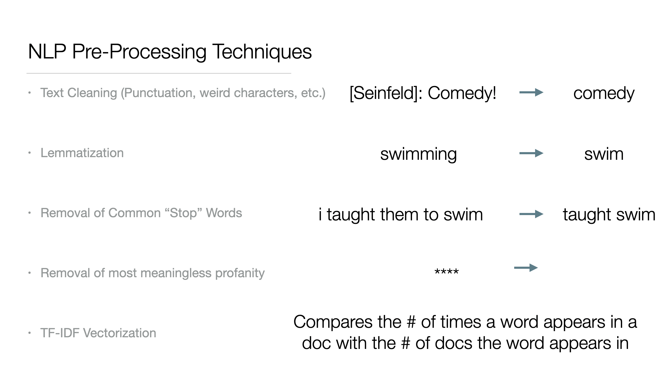Summary of text cleaning steps.

The final data format is “fit” on the initial dataset, and then applied to any incoming data (as is the case with the search engine feature described later in this post.)

To elaborate a bit on vectorization: I focused on trying out two types/implementations of vectorization in scikit-learn:

1. Count Vectorizer, which simply counts the frequency of each word in each document/transcript.
2. TF-IDF Vectorizer, which calculates the product of term frequency with its inverse-document frequency (a scale of 0 to 1 where values closer to zero are common in the entire dataset of transcripts). This is a valuable metric because it weights words that are common in a document more heavily if they aren’t common in general, which is a useful tool for ultimately extracting distinct topics.

In general, creating this pipeline was an iterative process. I tried out different transformations and did topic modeling (explained in the next section) to evaluate the effectiveness of different components in the pipeline. This helped inform my decision to vectorize the text with TF-IDF, as it yielded topics that were much more discernible and easy to label by looking at each topic’s top words.

One other note important note is that using pre-built lists of common English stop words to remove from the dataset isn’t a complete solution. I had to do quite a bit of combing through the transcripts to identify insignificant, yet common words and manually add them to the stop words list. It may come as no surprise that curse words are extremely prevalent in comedy, and don’t usually add much meaning, so I had to include some pretty aggressive words in my code (several of which are fairly offensive and I wouldn’t use in conversation).

Aside from also removing names/other irrelevant proper nouns, I also had to carefully decide what to do about racial slurs. Like it or not, racial slurs are common in stand-up comedy and can sometimes carry important meaning with regards to a comedian’s jokes. As a result, I left many of them in the dataset, but was also tasked with the uncomfortable task of hard-coding some extremely antiquated language in the NLP pipeline class for removal.

Modeling & Flask App Features

My main objective for this project was to develop a Flask application that provided more nuanced recommendations of comedy specials than what’s currently available on mainstream streaming platforms. I scoped out two features:

1. A dropdown genre filter using genres that were created by machine learning algorithms (as opposed to human labeling.)
2. A search bar that allows a user to describe the comedy they want to see, and get content-based recommendations.

You can play around with the app here.

Automatic Genre Filters with Topic Modeling

Creating machine-learned genres involves first applying the unsupervised learning technique of topic modeling, transforming the resulting data to extract which words are most closely related with each topic, and then performing the manual task of giving each topic a reasonable label.

In relatively simple terms, topic modeling involves reducing the dimensions of the document-term matrix (words) to a specified number of columns (representing the topics, and a weighting for each topic to each document). I tried a few different dimensionality reduction techniques including Latent Semantic Analysis (LSA), Latent Dirichlet Allocation (LDA), and Non-Negative Matrix Factorization (NMF). Ultimately, the scikit-learn implementation of NMF yielded the most discernible topics.

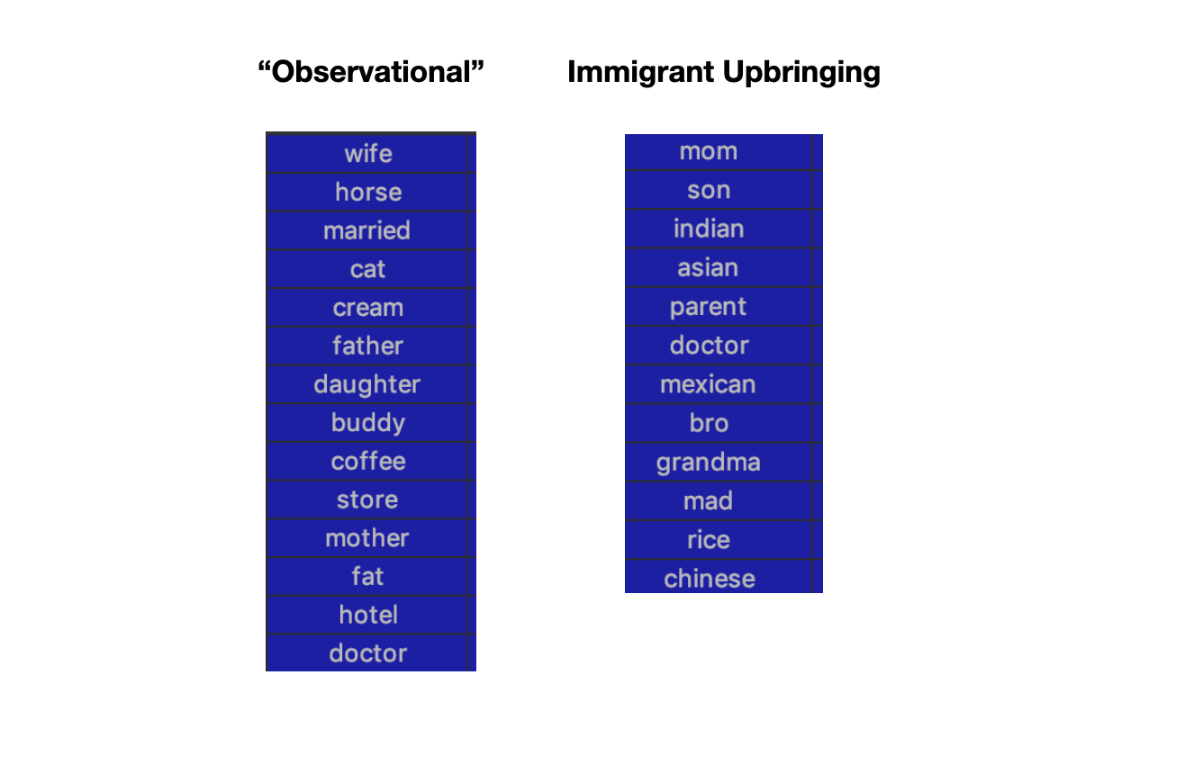Examples of top words associated with modeled topics.

Based on the top words generated from each topic, I used my knowledge of comedy to select the following genres:

• Observational: This is sort of a catch-all for “average”, “every day” topics such as family, chores, marriage, pets, etc. This type of comedy is quite common.
• Immigrant Upbringing: Many comedians are 1st generation Americans with parents that immigrated to the US and brought their culture with them. Comedians with recently immigrated families often talk about the humorous struggles of assimilation, the quirks of their various cultures, the pressures of their parents, and hardworking nature of their families.
• Relationships & Sex: This is another very common topic in comedy, particularly for “dirty” comedians. The sub-topics range from dating, to LGBTQ humor, and heavily sexual jokes.
• British/Australian: This topic was selected almost entirely based on colloquialisms of the comedian. While the United Kingdom and Australia have different cultures, they share some slang in common. If I were to continue to spend time on this project, I would probably try and separate these two topics, as British comedy historically is associate with a specific type of “dry” humor. That being said, many non-American english-speaking comedians share a common tendency to have more solid “themes” in their comedy specials as opposed to a random assortment of jokes.
• The Black Experience: I put a decent amount of effort into being sensitive around this topic. (Coincidentally, I was working on this project during the height of the protests in the wake of the murder of George Floyd by police in Minneapolis). Traditionally, Black comedians have been lumped into the genre of “Urban” comedy. While the “Urban” comedy scene is extremely rich in culture, that word seems to exist as an unnecessary euphemism. It is important to consider how a machine learning algorithm might be biased in a way that might marginalize groups of people. Additionally, I recognize that there is no such thing as a “monolithic black experience” - every individual has their own experience. All that being said, I still felt that this was a valid genre since Black Americans have collectively experienced many things throughout history from slavery, to segregation, to police brutality (and everything in between). And most impressively Black comedians have turned these issues and events on their head through humor and comedy to create dialogue (while entertaining people).

An important technical note here is that these genres are not exclusive to each comedy special in the data set - a comedy transcript can belong to multiple genres. Each comedy special is assigned a weight for each topic/genre, and considered “belonging” to that genre if the weight is above some threshold.

I put the genres in a dropdown menu in the Flask application. When a user selects a genre, Javascript code runs to filter out any comedy specials that are below a topic weight threshold of 0.2 for that genre.

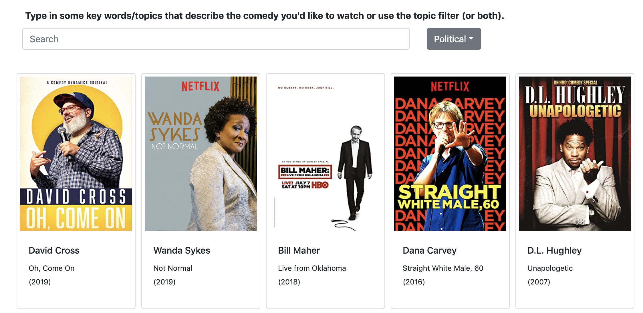Filtering comedy by genres generated through topic modeling.

Search Engine Recommender with Content-Based Filtering

The second feature was an opportunity for me to build my first recommender system with content-based filtering. My Flask app doesn’t have a large user base or any sort of “rating” functionality, so obviously collaborative filtering was not an option.

Search term recommender with content-based filtering

The main input to the recommender is a text field for which the user is asked to describe the type of comedy they want to see. When the user submits the text, it is treated similarly to a document from the main corpus: cleaned, transformed, and vectorized to the same format. It is then transformed using the NMF pre-fit on the comedy transcript corpus and assigned weights for each of the five topics.

Finally, the cosine similarity is calculated between the search term topic weights and each document (comedy special) in the transcript’s topic weights. The top 10 comedy specials with the largest cosine similarity with respect to the search term are recommended to the user.

Final Thoughts

Before learning about NLP or working on this project, I never thought of language as something that can be broken down, quantified, and processed by linear algebra. However, by using mathematical techniques and allowing a computer to determine patterns in human speech, we can learn a lot about how language works and what makes us laugh or identify with a particular set of thoughts.

This project also presented me with an ethical challenge when an unsupervised learning algorithm outputted comedy genres that fell within cultural and ethnic bounds. I got a lot out of learning to carefully navigate sensitive words, topics, and potential algorithmic bias.